Perfect! You’re thinking like a data analyst already — treating learning as a project-based journey. This approach will not only help you learn R deeply, but also produce a polished portfolio piece. Let’s begin.

---

🎯 Project Goal

Analyze supermarket sales data to uncover customer trends, product performance, and store dynamics.
Final output: a clean R Markdown report / Shiny dashboard with insights and visuals.

---

🧭 Project Outline: Supermarket Sales Analysis

Each stage improves a core data skill — think of it like a real client project.

---

Step 1: Understand the Dataset

🔍 Goal: Become familiar with what’s inside.

• Look at the column names: What do they represent? Which ones are categorical vs numeric?

• Try str() or glimpse() in R.

• How many rows? Any missing data?

• Can you guess what each row represents — a single purchase, an invoice, a daily summary?

📌 Hint: Use unique(), summary() and check table() for categorical variables.

---

Step 2: Clean and Prepare the Data

🧹 Goal: Make the dataset analysis-ready.

• Look for missing values or strange entries (e.g., “0” as tax or total).

• Convert date/time columns to proper Date or POSIXct format.

• Ensure numeric columns are really numeric.

• Consider feature engineering: e.g., extracting weekday, hour, or month.

📌 Hint: Use mutate(), as.Date(), and lubridate::wday().

---

Step 3: Exploratory Data Analysis (EDA)

📊 Goal: Discover patterns, answer business questions.

You’ll create a question list like:

• What are the busiest times of day / week / month?

• Which product lines bring in the most revenue?

• Which city/store performs best?

• Any interesting trends in payment method or customer type?

Start simple:

• Count plots for categories (bar charts)

• Histograms or density plots for totals

• Boxplots for comparing revenue across groups

📌 Hint: Use ggplot2 + dplyr. Think: group_by() → summarise() → ggplot().

---

Step 4: Segment the Customers

🧠 Goal: Understand different customer behaviors.

Choose one or two segmentation logics:

• By customer type (member vs normal)

• By spending pattern

• By purchase frequency (daily, weekday/weekend)

Can you calculate metrics like:

• Average purchase amount per group?

• Most popular product line per customer type?

📌 Hint: Use facet_wrap() to split plots. Try grouping by customer and summarizing.

---

Step 5: Build a Dashboard or Report

📦 Goal: Communicate your findings.

You now translate analysis into a portfolio artifact:

• R Markdown report: Clean layout with intro, methods, plots, insights.

• Shiny App (optional): Interactive dashboard with filters and charts.

• Add narrative! Why is this insight valuable?

📌 Hint: Structure your markdown with ##, include charts, use kable() for tables.

---

Step 6: Polish for Portfolio

📝 Goal: Make it readable, beautiful, and shareable.

• Add a project title, description, and motivation.

• Reflect briefly on: what you learned? what surprised you?

• Export as HTML/PDF (or deploy Shiny).

• Optional: Upload to GitHub or create an Obsidian note for your project log.

---

🧱 Skills You’ll Practice

• Tidyverse (dplyr, ggplot2, lubridate)

• Data cleaning

• EDA

• Data storytelling

• Report creation or dashboarding

---

Step 1: Understand the Dataset

1.1 Check the structure

library(tidyverse)
df <- read_csv("SuperMarket Analysis.csv")
head(df)
glimpse(df)
str(df)
names(df)
view(df)
dim(df)

1.2 Any obvious issues?

 
summary(df)
duplicated(df)
summary(is.na(df))

1.3 Peek into Date and Time

sapply(df, class)
library(lubridate)
unique(df$Date)
df <- df %>%
  mutate(Date = mdy(Date))
summary(df$Date)
 

Step 1 Summary:

• Dataset has 1000 rows and 17 columns.
• Key columns and their types:
  • Categorical: City, Gender, Customer type, Product line, Payment
  • Numerical: Unit price, Quantity, Tax, Total, Rating
  • Date/Time: Date, Time
• No missing values.
• No duplicated rows.

1.4 🤔 What does “parsing Date” mean?:

Analogy:

Imagine your Date column is like a string saying "12/01/2024" — it looks like a date, but R treats it as just text. Parsing is the act of telling R:
🗣️ “Hey, this is not just text — this is a real calendar date!”

So R will convert it into a Date class object. Once it’s parsed, you can:

• Extract month, weekday, year using lubridate like month(), wday()

• Sort data by date

• Group by week/month

• Make time-series plots

🧩 How to Check if It Needs Parsing

You can run this:

sapply(df, class)

Then look at what R says for the "Date" column:

If you see:

• "character" → ✅ Yes, you need to parse it

• "factor" → ✅ Also yes — first convert to character, then parse

• "Date" → ❌ No parsing needed, already done

✅ How to Parse

If needed, use lubridate::dmy() or mdy() depending on the format.

library(lubridate)
df <- df %>%
  mutate(Date = dmy(Date))  # or mdy(Date) if month is first

To figure out whether to use dmy() or mdy(), just look at the actual values:

• "12/01/2024" → if it means 12 Jan → use dmy()

• if it means Jan 12 → use mdy()

---

Step 2: Data Cleaning + Feature Engineering

2.1 Clean and Normalize Categorical Variables

❓ Are category names consistent? Look at columns like City, Customer type, Gender, Product line, Payment.

df %>% 
  count(City) 
 
df %>% 
  count(Payment)
  
df %>% 
  count(Gender)
 
df %>% 
  count(`Product line`)
 
df %>% 
  count(`Customer type`)

2.2 Extract New Time-Based Features

df <- df %>% 
  mutate(
    hour = hour(Time),
    day_part = case_when(
      hour < 12 ~ "Morning",
      hour >= 12 & hour < 18 ~ "Afternoon",
      hour >= 18 ~ "Evening"
    ),
    weekday = wday(df$Date, label = TRUE, abbr = FALSE),
    month = month(df$Date, label = TRUE, abbr = FALSE)
  )
 

2.2.1 In R’s mutate():

mutate(new_column = some_transformation)

This says:

“Create a new column called new_column, and fill it with values calculated by some_transformation.”

2.2.2 ✅ label = TRUE — return weekday name, not number

By default, wday() gives you numbers:

wday("2024-06-10")
#> [1] 2   (if week starts on Sunday → Monday = 2)

But when you do:

wday(date, label = TRUE)

You get human-readable names like:

[1] "Mon" "Tue" "Wed" ...

✅ abbr = FALSE — use full names instead of abbreviations

This controls how long the labels are:

Setting	Output
abbr = TRUE (default)	“Mon”, “Tue”, “Wed”
abbr = FALSE	”Monday”, “Tuesday”, “Wednesday”

So if you want clean, full day names for plots or tables (e.g., for a dashboard), then:

wday(date, label = TRUE, abbr = FALSE)

is perfect — it gives "Monday", "Tuesday", etc.

2.3 Create Summary Variables

Bucket customers into “Low”, “Medium”, “High” spenders

q3 <- quantile(df$Sales, probs = 0.75)
q1 <- quantile(df$Sales, probs = 0.25)
df <- df %>%  
  mutate(
    price_per_item = Sales / Quantity, #Actual average paid per item (including tax).
    spending_category = case_when(
      Sales <= q1 ~ 'Low_Spender',
      Sales > q1 & Sales <= q3 ~ 'Medium_Spender',
      Sales > q3 ~ 'High_Spender'
    )
    
  ) 
df %>% 
  count(spending_category)

Step 2 Summary:

• Checked categories: City, Gender, Payment, etc. — all consistent.
• Created time features: hour, weekday, month, day_part (Morning/Afternoon/Evening).
• Added summary vars:
  • price_per_item = Sales / Quantity
  • spending_category (Low / Medium / High) using quantiles.
• Data looks clean, no major outliers.

---

Step 3: Exploratory Data Analysis (EDA)

3.1 Understand Overall Sales Patterns

• What’s the distribution of Sales?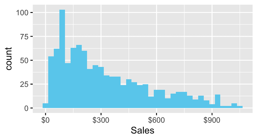

ggplot(df, aes(x = Sales)) +
  geom_histogram(binwidth = 30, fill = "skyblue") +
  scale_x_continuous(labels = scales::dollar)

• Which City performs best?

df %>% 
  group_by(City) %>% 
  summarise(
    avg_sales = mean(Sales, na.rm = TRUE)
  ) %>%
  slice_max(avg_sales)

• How does Payment method vary?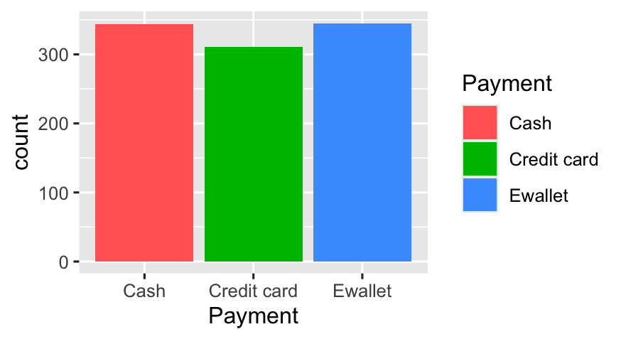

ggplot(df, aes(x = Payment, fill = Payment)) +
  geom_bar()

Goal	What you want to do	Correct Syntax
Use a fixed color (e.g., all bars red)	Not based on data	geom_bar(fill = "red")
Color based on a data variable (e.g., fill bars by Payment)	Based on a column in your data	aes(fill = Payment) inside ggplot()

---

3.2 Product & Customer Insights

• Which product_line earns the most revenue?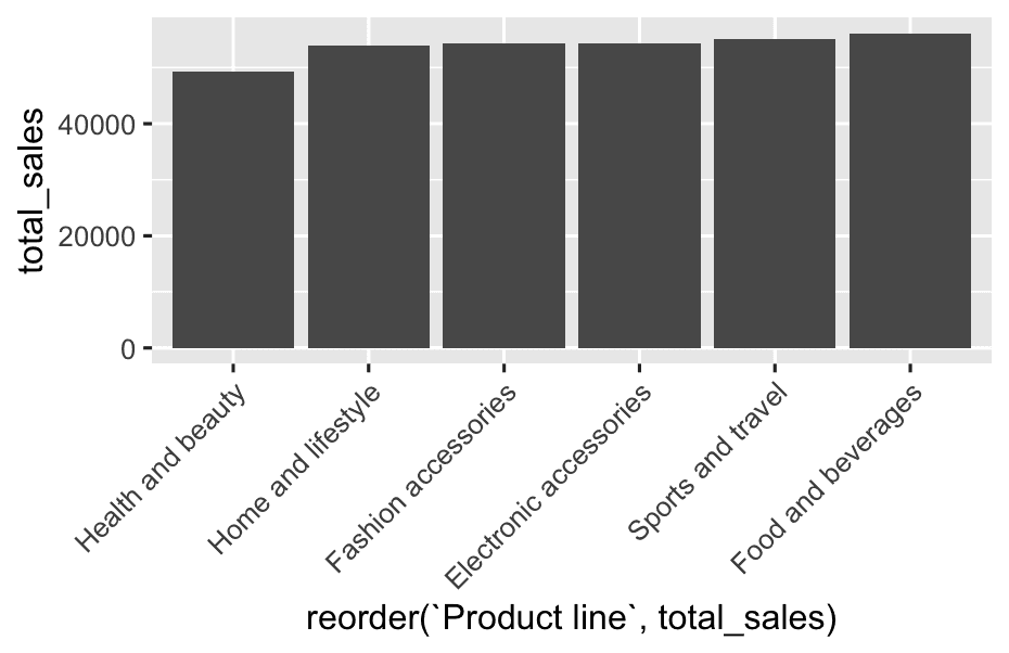

df %>% 
  group_by(`Product line`) %>% 
  summarise(
    total_sales = sum(Sales)
  ) %>%
  ggplot(aes(x = reorder(`Product line`, total_sales),y = total_sales)) +
  geom_col() +
  theme(axis.text.x = element_text(angle = 45,hjust=1))

• Are there differences by gender ?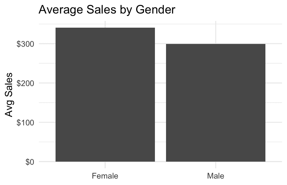

df %>% 
  group_by(Gender) %>% 
  summarise(
    avg_sales = mean(Sales, na.rm = TRUE)
  ) %>% 
  ggplot(aes(x = Gender,y = avg_sales)) +
  geom_bar(stat = "identity")+
  scale_y_continuous(labels = scales::dollar) +
  labs(title = "Average Sales by Gender", y = "Avg Sales", x = NULL) +
  theme_minimal()

• What’s the relationship between Quantity and Sales?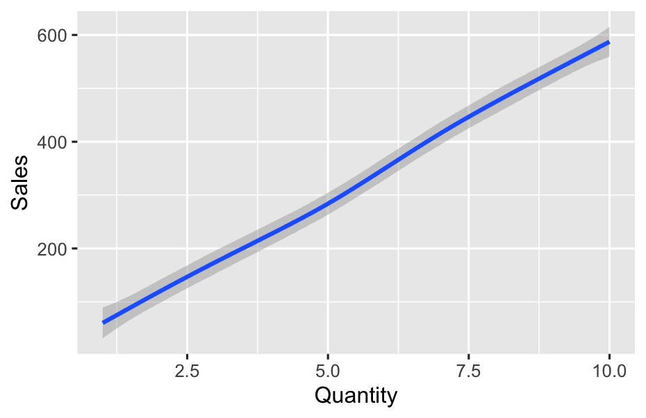

ggplot(df, aes(x = Quantity, y = Sales)) +
  geom_smooth()

---

3.3 Time Trends

• Which day_part or hour has higher sales?

df %>% 
  group_by(day_part) %>% 
  summarise(
    avg_sales = mean(Sales, na.rm = TRUE)
  ) %>% 
  slice_max(avg_sales)

• Do weekdays affect spending?

Key Concept: geom_bar(stat = "identity")

What it expects:

It needs your data to be already summarized — one row per bar.

But in your code:

ggplot(df, aes(x = weekday, y = Sales)) +
  geom_bar(stat = "identity")

You’re passing the full dataset (df) — not grouped yet.

So R tries to draw one bar per row, and uses the Sales in each row → this gives chaotic results or duplicates.

The Fix: summarise before plotting

Here’s the correct approach:

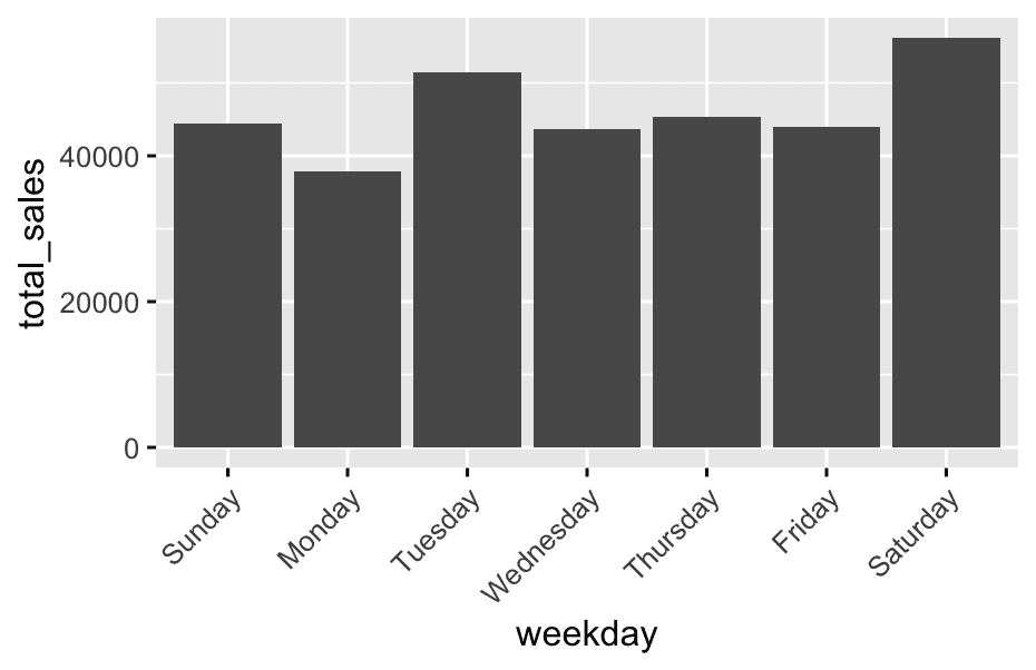
df %>%
  group_by(weekday) %>%
  summarise(total_sales = sum(Sales)) %>%
  ggplot(aes(x = weekday, y = total_sales)) +
  geom_col() +
  theme(axis.text.x = element_text(angle = 45,hjust=1))

This:

1. Groups data by weekday

2. Summarizes into one row per weekday with total sales

3. Passes that clean summary to ggplot

4. Uses geom_col() to plot bars where height = total_sales

✅ geom_col() is just a shortcut for:

“I already summarized my data — use these y-values directly.”

Step 4: Segment the Customers

4.1 By Customer Type (Member vs Normal)

• Is there a difference in preferred product lines or payment method?

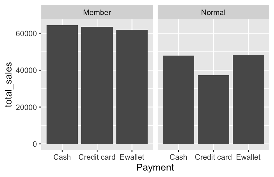
df %>%
  group_by(`Customer type`, Payment) %>%
  summarise(total_sales = sum(Sales), .groups = 'drop') %>%
  ggplot(aes(x = Payment, y = total_sales)) +
  geom_col() + 
  facet_wrap(~`Customer type`)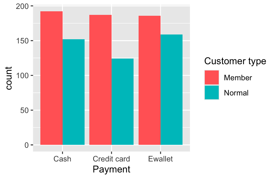

ggplot(df, aes(x = Payment, fill = `Customer type`)) +
  geom_bar(position = "dodge")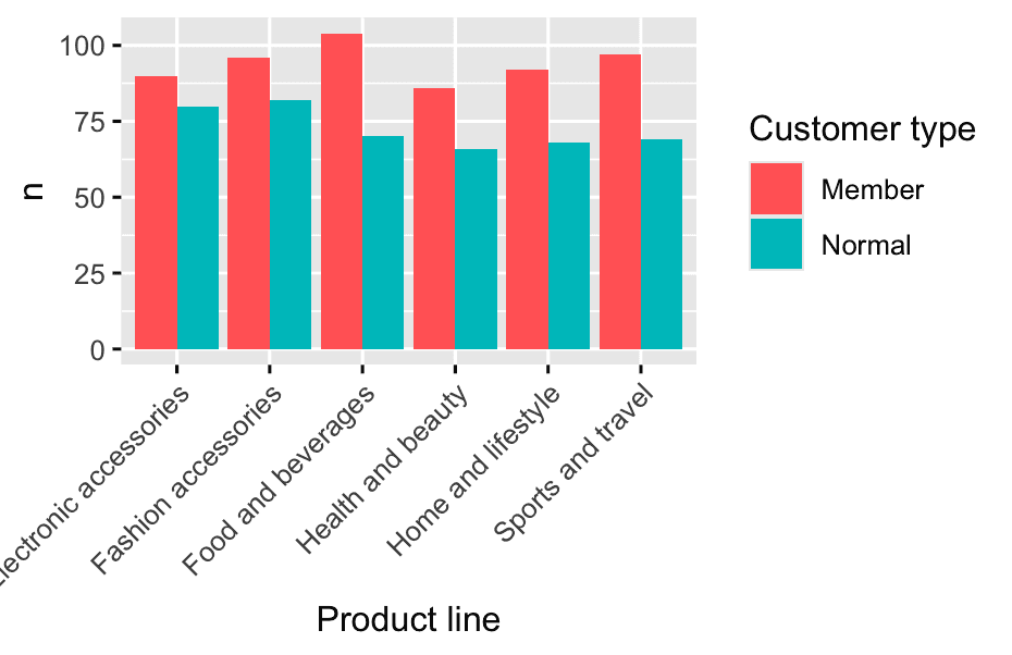

df %>% 
  count(`Customer type`, `Product line`) %>%
  ggplot(aes(x = `Product line`, y = n, fill = `Customer type`)) +
  geom_col(position = "dodge") +
  theme(axis.text.x = element_text(angle = 45, hjust = 1))
 

I made a mistake: You used:

df %>% 
  count(`Customer type`,`Product line`) %>% 
  ggplot(aes(x = `Product line`, fill = `Customer type`)) +
  geom_bar(position = "dodge")

But geom_bar() with pre-counted data (after count()) defaults to counting the number of rows — not using your actual counts!
Since your summary table already has the counts (n), every bar just shows “1”.

How to fix it: Use geom_col() instead of geom_bar():

geom_col() uses the height of bars from your n column:

df %>% 
  count(`Customer type`, `Product line`) %>%
  ggplot(aes(x = `Product line`, y = n, fill = `Customer type`)) +
  geom_col(position = "dodge") +
  theme(axis.text.x = element_text(angle = 45, hjust = 1))

Now you’ll see the actual transaction count for each product line by customer type.

Key rule:

• After summarizing/counting: Use geom_col() with y = n

• Raw data, want counts: Use geom_bar()

4.2 By Spending Pattern (Low / Medium / High Spender)

• How do “high spenders” behave differently? Do they favor certain products, times, or payment types? 1️⃣ Raw count of high spender transactions by product line

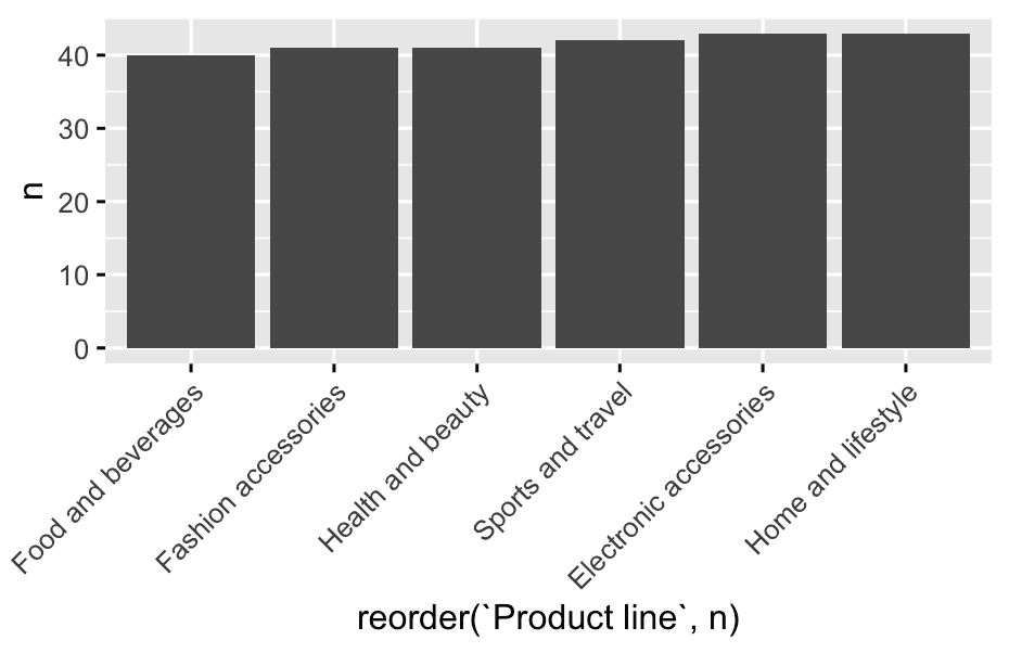
df %>%
  filter(spending_category == 'High_Spender') %>%
  count(`Product line`) %>%
  ggplot(aes(reorder(`Product line`, n),y = n)) +
  geom_col(position = "dodge") +
  theme(axis.text.x = element_text(angle = 45, hjust = 1))
 

2️⃣ Percentage of high spenders by product line

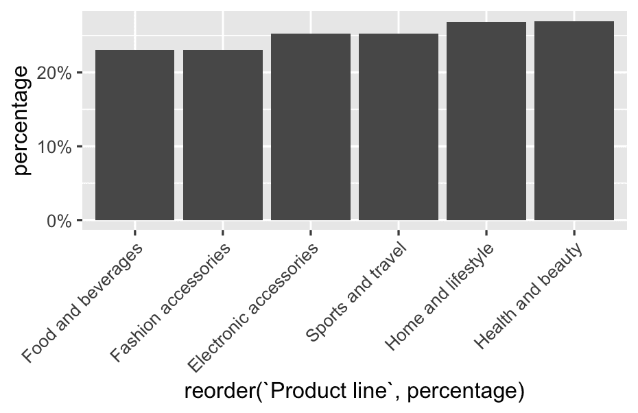
product_totals <- df %>%
  count(`Product line`, name = "total_count")
high_spender_totals <- df %>%
  filter(spending_category == "High_Spender") %>%
  count(`Product line`, name = "high_spender_count")
final_table <- left_join(product_totals, high_spender_totals, by = "Product line")
final_table %>% 
  mutate(
    percentage = high_spender_count / total_count
  ) %>% 
  ggplot( aes(reorder(`Product line`, percentage), y = percentage)) +
  geom_col() +
  scale_y_continuous(labels = scales::percent_format(accuracy = 1)) +
  theme(axis.text.x = element_text(angle = 45, hjust = 1))

4.3 By Purchase Frequency (Day, Weekday/Weekend)

• Do some customers shop more on weekends?

Number of Transactions: Weekend vs Weekday:

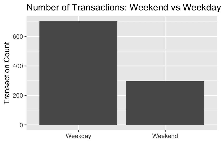
df <- df %>%
  mutate(
    weekpart = case_when(
      weekday == 'Saturday' | weekday == 'Sunday' ~ "Weekend",
      TRUE ~ "Weekday"
    )
  )
 
df %>% 
  count(weekpart) %>% 
  ggplot(aes(x = weekpart, y = n)) +
  geom_col(position = "dodge") +
  labs(
    title = "Number of Transactions: Weekend vs Weekday",
    x = NULL,
    y = "Transaction Count"
  ) 

TRUE ~ "Weekday"
For all other rows, set weekpart to "Weekday".

Average Sales per Transaction: Weekend vs Weekday:

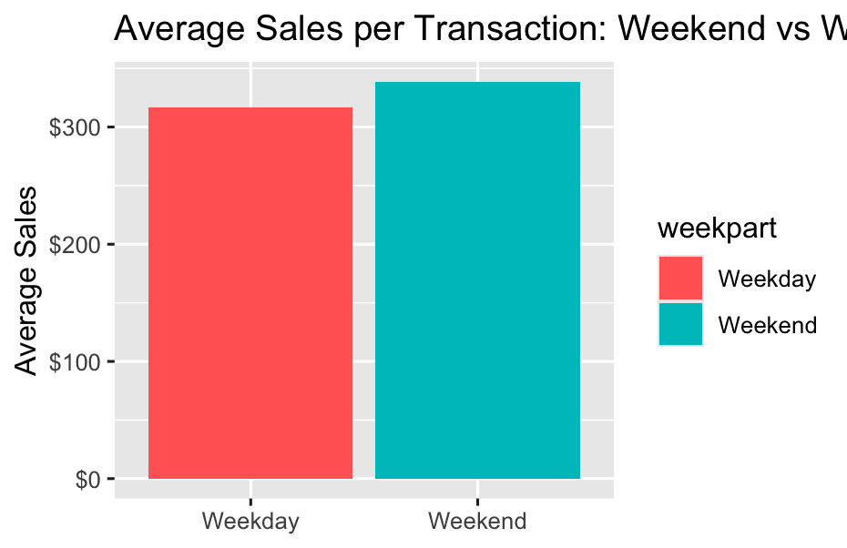
df %>% 
  group_by(weekpart) %>% 
  summarise(avg_sales = mean(Sales, na.rm = TRUE)) %>% 
  ggplot(aes(x = weekpart, y = avg_sales, fill = weekpart)) +
  geom_col() +
  scale_y_continuous(labels = scales::dollar) +
  labs(
    title = "Average Sales per Transaction: Weekend vs Weekday",
    x = NULL,
    y = "Average Sales"
  ) 

• Are high spenders more “weekend” or “weekday”?

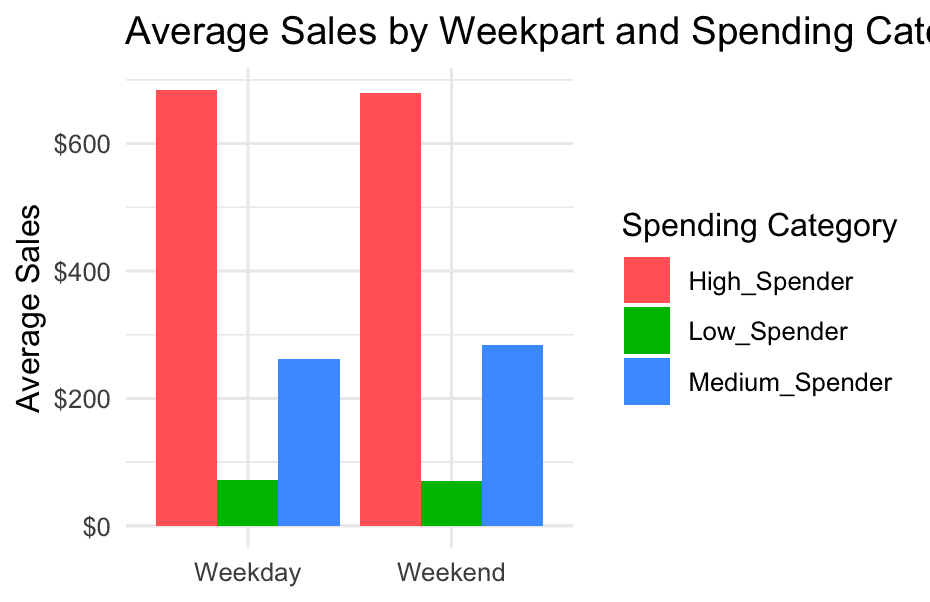
df %>%
  group_by(weekpart, spending_category) %>%
  summarise(avg_sales = mean(Sales, na.rm = TRUE)) %>%
  ggplot(aes(x = weekpart, y = avg_sales, fill = spending_category)) +
  geom_col(position = "dodge") + 
  labs(title = "Average Sales by Weekpart and Spending Category", x = NULL, y = "Average Sales") +
  scale_y_continuous(labels = scales::dollar) +
  scale_fill_discrete(name = "Spending Category") +
  theme_minimal()