Linear Regression - Polynomial Regression

2025-10-30 18:04 Tags:

Overview

In simple linear regression, we fit a straight line to data.
Now, we’ll extend that idea to handle non-linear relationships using polynomial regression.

Along the way, we’ll also discuss:

Overfitting and underfitting
Model evaluation
Choosing model complexity (polynomial degree)

Imports

import numpy as np
import pandas as pd
import matplotlib.pyplot as plt
import seaborn as sns

Sample Data

We’ll use the Advertising dataset from ISLR.

It shows sales (in thousands of units) as a function of advertising budgets (in thousands of dollars) for TV, Radio, and Newspaper.

df = pd.read_csv("Advertising.csv")
df.head()
 
X = df.drop('sales', axis=1)
y = df['sales']

Polynomial Features

We can create new polynomial features using PolynomialFeatures from sklearn.preprocessing.

Example for one feature:

\overset{y}{^} = β_{0} + β_{1} x + ϵ

becomes

\overset{y}{^} = β_{0} + β_{1} x + β_{2} x^{2} + \dots + β_{d} x^{d} + ϵ

Multiple Features Case

If an input sample has multiple features [a, b] and we choose degree = 2,
then new polynomial features will include:

$[1, a, b, a^{2}, ab, b^{2}]$

Example:

from sklearn.preprocessing import PolynomialFeatures
 
polynomial_converter = PolynomialFeatures(degree=2, include_bias=False)
poly_features = polynomial_converter.fit_transform(X)
poly_features.shape

Interaction terms include:
$x_{1} x_{2}, x_{1} x_{3}, x_{2} x_{3}$

1️⃣ polynomial_converter = PolynomialFeatures(degree=2, include_bias=False)

This creates a tool (an object) that knows how to generate new polynomial features from your data.

degree=2 → means it will create terms like
( x_1^2, x_2^2, x_1x_2 ), etc.
include_bias=False → means we don’t add a column of all 1s (that’s the intercept term; the regression model handles it).

So polynomial_converter is like a recipe book for making new polynomial features.

2️⃣ .fit(X)

The fit() part means:

“Look at the structure of my input data X and remember how many features (columns) it has.”

Example:
If X has 3 columns — [TV, Radio, Newspaper] —
then the converter figures out how to combine them (squares, products, etc.) for degree 2.

It does not change or calculate anything yet — it just learns the pattern.

3️⃣ .transform(X)

Now it actually creates new columns based on that pattern.

For degree=2 and 3 features (x₁, x₂, x₃), it will produce:

Original Features	New Polynomial Features
x₁, x₂, x₃	x₁, x₂, x₃, x₁², x₂², x₃², x₁x₂, x₁x₃, x₂x₃

So if you had 3 features before, you’ll now have 9 columns in total.

4️⃣ .fit_transform(X)

This is just a shortcut:
instead of calling .fit(X) and then .transform(X) separately,
it does both in one step.

So effectively:

polynomial_converter.fit(X)
poly_features = polynomial_converter.transform(X)

is the same as:

poly_features = polynomial_converter.fit_transform(X)

poly_features.shape

(200, 9)

X.shape

(200, 3)

X.iloc[0]

TV 230.1 radio 37.8 newspaper 69.2 Name: 0, dtype: float64

poly_features[0][:3]

array([230.1, 37.8, 69.2])

Train | Test Split

We split the dataset to evaluate model performance fairly.

from sklearn.model_selection import train_test_split
 
X_train, X_test, y_train, y_test = train_test_split(
    poly_features, y, test_size=0.3, random_state=101
)

Model Fitting

We can fit a simple Linear Regression model on the transformed polynomial data.

from sklearn.linear_model import LinearRegression
 
model = LinearRegression(fit_intercept=True)
model.fit(X_train, y_train)

Model Evaluation

Evaluate performance on unseen (test) data.

from sklearn.metrics import mean_absolute_error, mean_squared_error
 
test_predictions = model.predict(X_test)
MAE = mean_absolute_error(y_test, test_predictions)
MSE = mean_squared_error(y_test, test_predictions)
RMSE = np.sqrt(MSE)

Choosing Model Complexity

We can experiment with different polynomial degrees to detect overfitting. Let’s use a for loop to do the following:

Create different order polynomial X data
Split that polynomial data for train/test
Fit on the training data
Report back the metrics on both the train and test results
Plot these results and explore overfitting

# TRAINING ERROR PER DEGREE
 
train_rmse_errors = []
 
# TEST ERROR PER DEGREE
 
test_rmse_errors = []
 
  
 
for d in range(1,10):
 
# CREATE POLY DATA SET FOR DEGREE "d"
 
polynomial_converter = PolynomialFeatures(degree=d,include_bias=False)
 
poly_features = polynomial_converter.fit_transform(X)
 
# SPLIT THIS NEW POLY DATA SET
 
X_train, X_test, y_train, y_test = train_test_split(poly_features, y, test_size=0.3, random_state=101)
 
# TRAIN ON THIS NEW POLY SET
 
model = LinearRegression(fit_intercept=True)
 
model.fit(X_train,y_train)
 
# PREDICT ON BOTH TRAIN AND TEST
 
train_pred = model.predict(X_train)
 
test_pred = model.predict(X_test)
 
# Calculate Errors
 
# Errors on Train Set
 
train_RMSE = np.sqrt(mean_squared_error(y_train,train_pred))
 
# Errors on Test Set
 
test_RMSE = np.sqrt(mean_squared_error(y_test,test_pred))
 
  
 
# Append errors to lists for plotting later
 
train_rmse_errors.append(train_RMSE)
 
test_rmse_errors.append(test_RMSE)

Plot RMSE vs. Polynomial Degree

plt.plot(range(1,6),train_rmse_error[:5],label='TRAIN')
 
plt.plot(range(1,6),test_rmse_errors[:5],label='TEST')
 
plt.xlabel("Polynomial Complexity")
 
plt.ylabel("rmse")
 
plt.legend()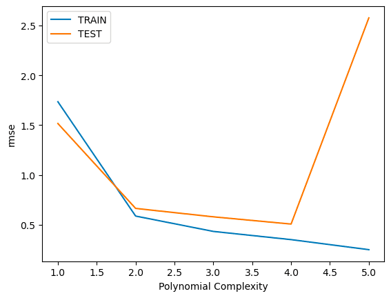

Pasted image 20251103195946.png

plt.plot(range(1,10), train_rmse_errors, label='TRAIN')
plt.plot(range(1,10), test_rmse_errors, label='TEST')
plt.xlabel("Polynomial Complexity (Degree)")
plt.ylabel("RMSE")
plt.legend()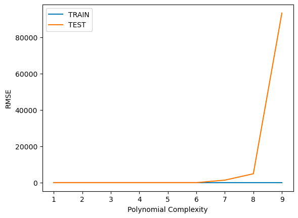

Pasted image 20251103195959.png

Final Model Selection

Based on test RMSE, we choose a degree = 3 model (safe side of complexity).

final_poly_converter = PolynomialFeatures(degree=3, include_bias=False)
final_model = LinearRegression()
 
final_model.fit(final_poly_converter.fit_transform(X), y)

Save the Model

from joblib import dump, load
 
dump(final_model, 'sales_poly_model.joblib')
dump(final_poly_converter, 'poly_converter.joblib')

Deployment and Predictions

When making new predictions, remember to transform the new data with the same converter.

loaded_poly = load('poly_converter.joblib')
loaded_model = load('sales_poly_model.joblib')
 
campaign = [[149, 22, 12]]
campaign_poly = loaded_poly.transform(campaign)
prediction = loaded_model.predict(campaign_poly)
print(prediction)

🪴LYC