2025-10-14 14:52 Tags:

📊 Dataset Overview

We use the Advertising dataset (from ISLR), showing:

• sales — units sold (in thousands)

• TV, radio, newspaper — advertising spend (in thousands of dollars)

df = pd.read_csv("Advertising.csv")
df.head()

We create a new variable:

df['total_spend'] = df['TV'] + df['radio'] + df['newspaper']

Then visualize:(that’s one way to know their relationship)

sns.scatterplot(x='total_spend', y='sales', data=df)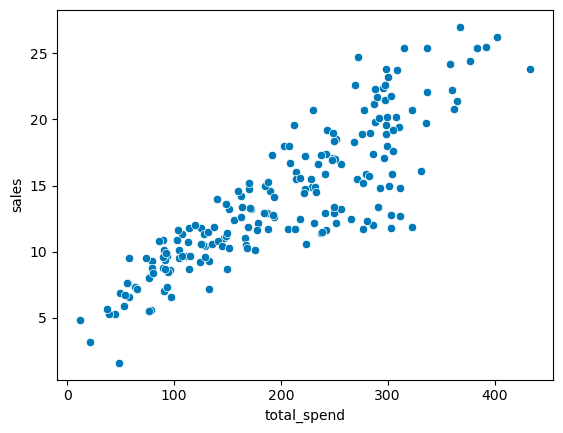

sns.regplot(x='total_spend',y='sales',data=df)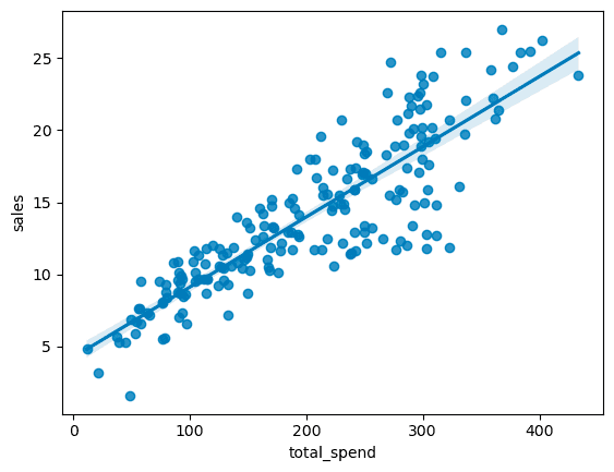

Is there a relationship between total advertising spend and sales?

---

📈 Least Squares Line

$y=mx+b$

$\hat{y}={\beta }_0+{\beta }_{1}X$

Using NumPy’s polyfit()

This is the function to solve beta0 and beta1

X = df['total_spend']
y = df['sales']
 
# Returns highest order coefficient first
np.polyfit(X, y, 1)

Example output:

array([0.04868788, 4.24302822])

So our regression line is:

$\hat{y}=0.0487X+4.243$

---

🔮 Predicting Future Sales

If a future campaign has a total spend of $200k:

spend = 200
predicted_sales = 0.04868788 * spend + 4.24302822
predicted_sales

Result:

Predicted sales ≈ 14.98 (thousand units)

Visualize the line:

potential_spend = np.linspace(0, 500, 100) # in total 100 points
predicted_sales = 0.04868788 * potential_spend + 4.24302822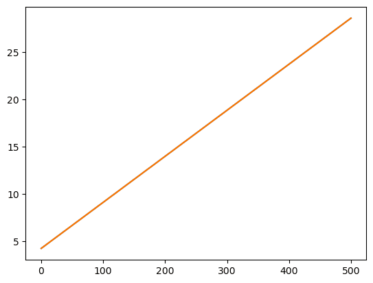

plt.plot(potential_spend, predicted_sales)

sns.scatterplot(x='total_spend', y='sales', data=df)
plt.plot(potential_spend, predicted_sales, color='red')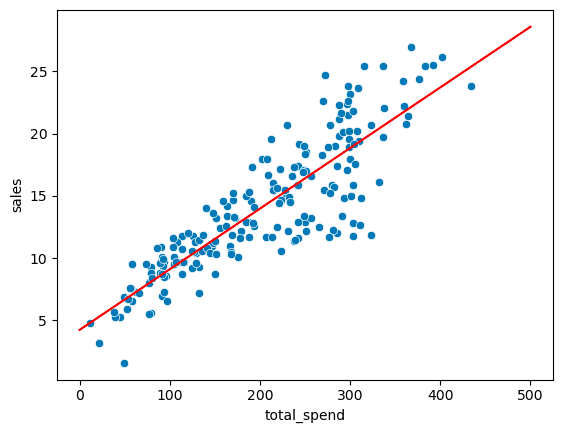

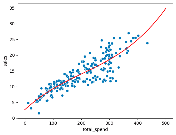
🔍 Model Fit and Complexity

We used a 1st-order polynomial (a straight line).
What happens if we try higher orders?

np.polyfit(X, y, 3)

array([ 3.07615033e-07, -1.89392449e-04, 8.20886302e-02, 2.70495053e+00]) y = B3x** 3 + B2x ** 2 + B1x + B0 The coefficients are quite small, which means they have very small effects, so not very reasonable here.

Produces a cubic model:

predicted_sales = (
    3.07615033e-07 * potential_spend**3
    - 1.89392449e-04 * potential_spend**2
    + 8.20886302e-02 * potential_spend
    + 2.70495053
)

sns.scatterplot(x='total_spend', y='sales', data=df)
plt.plot(potential_spend, predicted_sales, color='red')