5.3 Lengthening data

5.3.1 Data in column names

billboard
#> # A tibble: 317 × 79
#>   artist       track               date.entered   wk1   wk2   wk3   wk4   wk5
#>   <chr>        <chr>               <date>       <dbl> <dbl> <dbl> <dbl> <dbl>
#> 1 2 Pac        Baby Don't Cry (Ke… 2000-02-26      87    82    72    77    87
#> 2 2Ge+her      The Hardest Part O… 2000-09-02      91    87    92    NA    NA
#> 3 3 Doors Down Kryptonite          2000-04-08      81    70    68    67    66
#> 4 3 Doors Down Loser               2000-10-21      76    76    72    69    67
#> 5 504 Boyz     Wobble Wobble       2000-04-15      57    34    25    17    17
#> 6 98^0         Give Me Just One N… 2000-08-19      51    39    34    26    26
#> # ℹ 311 more rows
#> # ℹ 71 more variables: wk6 <dbl>, wk7 <dbl>, wk8 <dbl>, wk9 <dbl>, …

billboard %>% 
  pivot_longer(
    cols = starts_with('wk'),
    names_to = 'week',
    values_to = 'rank'
    values_drop_na = TRUE
  )

• cols specifies which columns need to be pivoted, i.e. which columns aren’t variables. This argument uses the same syntax as select() so here we could use !c(artist, track, date.entered) or starts_with("wk").
• names_to names the variable stored in the column names, we named that variable week.
• values_to names the variable stored in the cell values, we named that variable rank.
• This data is now tidy, but we could make future computation a bit easier by converting values of week from character strings to numbers using mutate() and readr::parse_number(). parse_number() is a handy function that will extract the first number from a string, ignoring all other text.

billboard %>% 
  pivot_longer(
    cols = starts_with('wk'),
    names_to = 'week',
    values_to = 'rank',
    values_drop_na = TRUE
  ) %>% 
  mutate(
    week  = parse_number(week)
  )

# A tibble: 5,307 × 5
   artist  track                   date.entered  week  rank
   <chr>   <chr>                   <date>       <dbl> <dbl>
 1 2 Pac   Baby Don't Cry (Keep... 2000-02-26       1    87
 2 2 Pac   Baby Don't Cry (Keep... 2000-02-26       2    82
 3 2 Pac   Baby Don't Cry (Keep... 2000-02-26       3    72
 4 2 Pac   Baby Don't Cry (Keep... 2000-02-26       4    77
 5 2 Pac   Baby Don't Cry (Keep... 2000-02-26       5    87
 6 2 Pac   Baby Don't Cry (Keep... 2000-02-26       6    94
 7 2 Pac   Baby Don't Cry (Keep... 2000-02-26       7    99
 8 2Ge+her The Hardest Part Of ... 2000-09-02       1    91
 9 2Ge+her The Hardest Part Of ... 2000-09-02       2    87
10 2Ge+her The Hardest Part Of ... 2000-09-02       3    92
# ℹ 5,297 more rows
# ℹ Use `print(n = ...)` to see more rows
> 

🧠 What does parse_number() do?

It comes from the readr package (part of the tidyverse). Its job is to:

Extract numbers from a character string

✅ It keeps the number
❌ It removes all non-numeric characters (like “Week”, “wk”, etc.)

billboard_longer %>% 
  ggplot(aes(x=week,y=rank,group=track)) +
  geom_line(alpha = 0.25)
  scale_y_reverse()

🧠 Why scale_y_reverse()?

Because Billboard chart rankings are reversed:

• Rank 1 is the best

• Rank 100 is the worst

We reverse the y-axis to make better rankings appear higher, which is more intuitive.

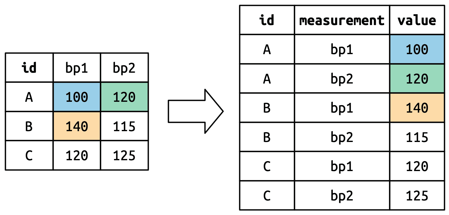
5.3.2 How does pivoting work?

  df <- tribble(
    ~id,  ~bp1, ~bp2,
    "A",  100,  120,
    "B",  140,  115,
    "C",  120,  125
  )
  
df %>% 
  pivot_longer(
    cols = bp1:bp2,
    names_to = 'measurement',
    values_to = 'value'
  )

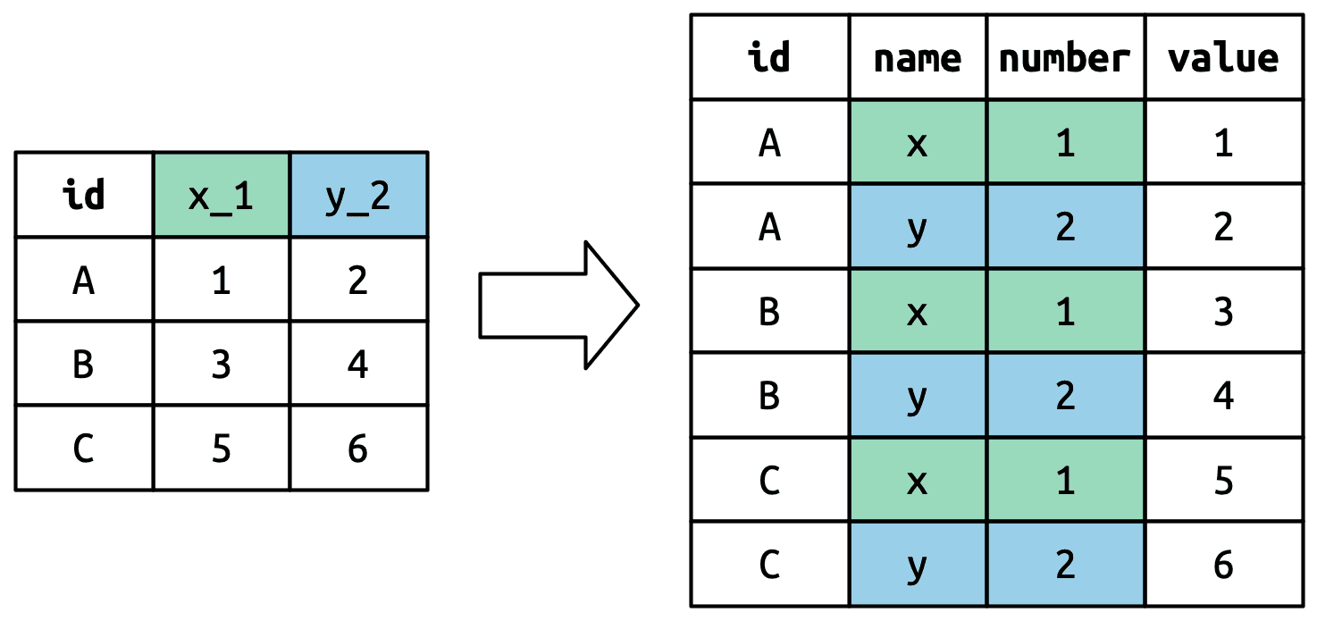
5.3.3 Many variables in column names

who %>% 
  pivot_longer(
    cols = !(country:year),
    names_to = c('dignosis','gender','age'),
    names_sep = '_',
    values_to = 'count'
  )

🔍 What does names_sep = "_" mean?

“When splitting column names into multiple variables using names_to, split them wherever there’s an underscore (_).”

5.3.4 Data and variable names in the column headers

household
#> # A tibble: 5 × 5
#>   family dob_child1 dob_child2 name_child1 name_child2
#>    <int> <date>     <date>     <chr>       <chr>      
#> 1      1 1998-11-26 2000-01-29 Susan       Jose       
#> 2      2 1996-06-22 NA         Mark        <NA>       
#> 3      3 2002-07-11 2004-04-05 Sam         Seth       
#> 4      4 2004-10-10 2009-08-27 Craig       Khai       
#> 5      5 2000-12-05 2005-02-28 Parker      Gracie

household %>% 
  pivot_longer(
    cols = !family,
    names_to = c('.value','child'),
    names_sep = '_',
    values_drop_na = TRUE
  )
 
#> # A tibble: 9 × 4
#>   family child  dob        name 
#>    <int> <chr>  <date>     <chr>
#> 1      1 child1 1998-11-26 Susan
#> 2      1 child2 2000-01-29 Jose 
#> 3      2 child1 1996-06-22 Mark 
#> 4      3 child1 2002-07-11 Sam  
#> 5      3 child2 2004-04-05 Seth 
#> 6      4 child1 2004-10-10 Craig
#> # ℹ 3 more rows

I am confused about .value, so I asked Gpt to fully explain it to me:

🧠 First: What does pivot_longer() usually do?

By default, it takes many columns and turns them into two columns:

• One for the column name (like name)

• One for the value (like Susan)

---

🌰 Mini example:

Original:

id	name_A	name_B
1	Alice	Bob

Usual pivot_longer() (no .value):

pivot_longer(cols = starts_with("name"),
             names_to = "key",
             values_to = "value")

✅ You get:

id	key	value
1	name_A	Alice
1	name_B	Bob

So everything goes into one value column — regardless of what type of data it is.

---

🤯 But what if… we had different kinds of variables in the columns?

Like in your case:

| family | dob_child1 | dob_child2 | name_child1 | name_child2 |

Now the column names contain two pieces of info:

1. The type of variable: dob or name

2. The child number: child1 or child2

---

🧱 Option A: Without .value

pivot_longer(
  cols = -family,
  names_to = c("what", "child"),
  names_sep = "_"
)

Gives you:

family	what	child	value
1	dob	child1	1998-11-26
1	name	child1	Susan
1	dob	child2	2000-01-29
1	name	child2	Jose

This is a long, stacked format. Everything is in one value column. You’d have to pivot_wider() again later to separate dob and name.

---

✅ Option B: With .value

pivot_longer(
  cols = -family,
  names_to = c(".value", "child"),
  names_sep = "_"
)

This says:

“Use the first part of the column name (like dob, name) as the name of a new column, and the second part (child1, child2) as a grouping variable.”

Now you get:

family	child	dob	name
1	child1	1998-11-26	Susan
1	child2	2000-01-29	Jose

Now it’s tidy:

• Each row is a child

• dob and name are separate columns, not stacked

---

🎯 So why use .value?

Because you want different pieces of the original column names to become different columns, not all shoved under a single “value”.

With .value	Without .value
You get multiple value columns	You get one stacked value column
Easier to use directly (tidy)	Often need to pivot_wider() later
Each row = one observation (e.g. child)	Each row = one variable of one child

---

5.4 Widening data

So far we’ve used pivot_longer() to solve the common class of problems where values have ended up in column names. Next we’ll pivot (HA HA) to pivot_wider(), which makes datasets wider by increasing columns and reducing rows and helps when one observation is spread across multiple rows. This seems to arise less commonly in the wild, but it does seem to crop up a lot when dealing with governmental data.

cms_patient_experience
#> # A tibble: 500 × 5
#>   org_pac_id org_nm                     measure_cd   measure_title   prf_rate
#>   <chr>      <chr>                      <chr>        <chr>              <dbl>
#> 1 0446157747 USC CARE MEDICAL GROUP INC CAHPS_GRP_1  CAHPS for MIPS…       63
#> 2 0446157747 USC CARE MEDICAL GROUP INC CAHPS_GRP_2  CAHPS for MIPS…       87
#> 3 0446157747 USC CARE MEDICAL GROUP INC CAHPS_GRP_3  CAHPS for MIPS…       86
#> 4 0446157747 USC CARE MEDICAL GROUP INC CAHPS_GRP_5  CAHPS for MIPS…       57
#> 5 0446157747 USC CARE MEDICAL GROUP INC CAHPS_GRP_8  CAHPS for MIPS…       85
#> 6 0446157747 USC CARE MEDICAL GROUP INC CAHPS_GRP_12 CAHPS for MIPS…       24
#> # ℹ 494 more rows

cms_patient_experience %>% 
  pivot_wider(
    id_cols = starts_with('org'), 
    names_from = measure_cd,
    values_from = prf_rate
  )

id_cols = starts_with("org")

This tells R:

“Keep org_pac_id and org_nm as identifiers — don’t pivot them.”

Because you don’t want org names or IDs turning into new columns — they should stay on the left, like “row headers”.

names_from = measure_cd

This tells R:

“Use the unique values in measure_cd as the names of new columns.”

So CAHPS_GRP_1, CAHPS_GRP_2, CAHPS_GRP_3… become new column names.

5.4.1 How does pivot_wider() work?

I am confused by this sentence, so I ask gpt to explain it for me: By default, the rows in the output are determined by all the variables that aren’t going into the new names or values. These are called the id_cols

🤔 So… what should stay as the “row identifier” (id_cols)?

The rule is:

Any column that is not involved in names_from or values_from is used to group rows together — it defines one row in the new wide table.

In this case:

• measurement becomes column names

• value becomes column values

• So id is left over → it becomes the id_col that defines the rows

That means each unique id becomes a row in the result