
Analyzing movie ratings bias with real-world data.
🎬 Fandango Movie Rating Bias Analysis
🧠 Project Overview
How reliable are online movie ratings, especially when the platform profits from ticket sales?
Inspired by FiveThirtyEight’s investigation, this project dives deep into Fandango’s 2015 ratings to explore potential biases.
Through data cleaning, exploratory data analysis (EDA), cross-platform comparisons, and visual storytelling, the goal was to uncover whether Fandango systematically inflated its movie ratings.
📚 Background and Data
In 2015, FiveThirtyEight reported that Fandango’s displayed movie ratings were consistently higher than true user ratings.
To investigate this, two datasets were analyzed:
- fandango_scrape.csv: Displayed stars, true user ratings, and number of votes on Fandango.
- all_sites_scores.csv: Critic and user ratings from Rotten Tomatoes, Metacritic, and IMDb.
All data was scraped and publicly released by FiveThirtyEight.
🛠️ Tools and Skills
- Python (Pandas, NumPy)
- Exploratory Data Analysis (EDA)
- Data Cleaning and Feature Engineering
- Visualization (Seaborn, Matplotlib)
- Data Normalization and Platform Comparison
🔍 1. Data Cleaning and Preparation
Basic cleaning steps:
- Extracted the release year from movie titles.
- Removed movies with zero votes to focus on reviewed films.
- Created a new feature:
[STARS_DIFF = STARS - RATING]
to measure discrepancies between displayed ratings and true ratings.
Quick dataset preview:
fandango.head()
fandango.info()
fandango.describe()
🔎 2. Exploratory Data Analysis (EDA)
2.1 Votes vs Rating Scatterplot
Exploring the relationship between popularity and ratings:
import matplotlib.pyplot as plt
plt.figure(figsize=(12,8))
sns.scatterplot(x='RATING', y='VOTES', data=fandango)
plt.show()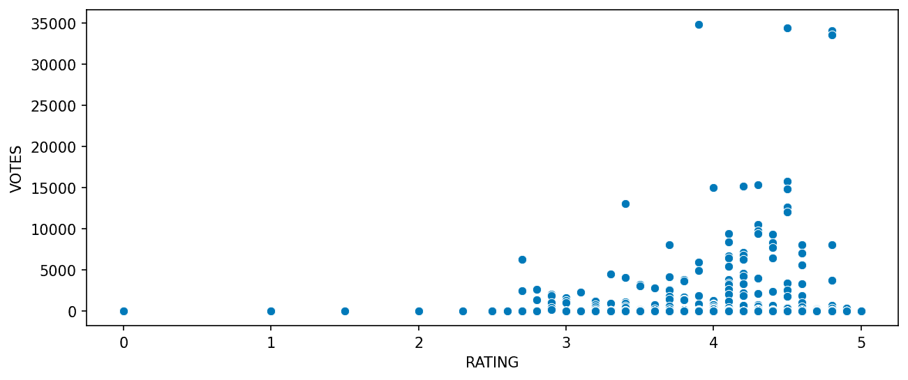 Popular movies tend to have higher ratings, but with significant variance.
2.2 Top 10 Movies by Number of Votes
Finding the most popular movies based on user votes:
fandango.nlargest(10, 'VOTES')[['FILM', 'VOTES', 'RATING'|'FILM', 'VOTES', 'RATING']]2.3 Movies with Zero Votes
Identifying movies that received no user votes:
fandango[fandango['VOTES'] == 0]
no_votes.sum()
🎯 3. Displayed Ratings vs True Ratings
3.1 KDE Plot Comparison
Visualizing distributions of displayed stars vs true user ratings:
plt.figure(figsize=(10,4),dpi=150)
sns.kdeplot(data=fan_reviewed,x='RATING',clip=[0,5],fill=True,label='True Rating')
sns.kdeplot(data=fan_reviewed,x='STARS',clip = [0,5],fill=True,label='Stars Displayed')
plt.legend(loc=(1.05,0.5))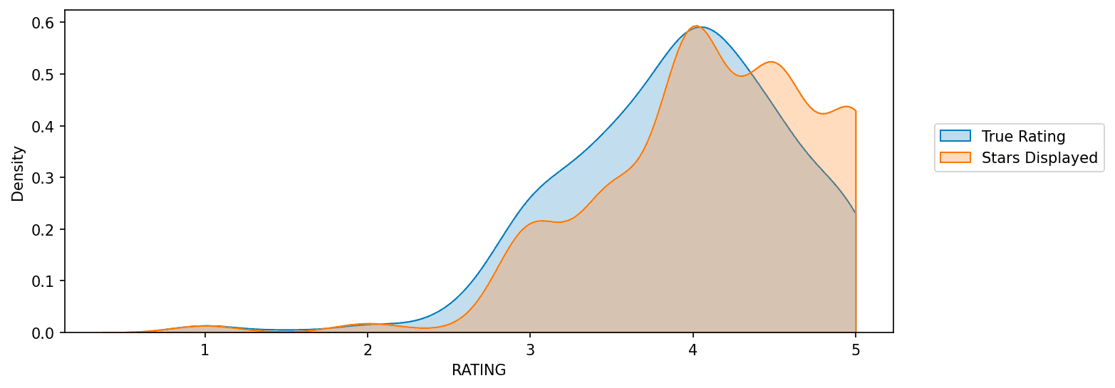
Displayed stars generally skew higher than actual ratings.
3.2 STARS_DIFF Distribution
Quantifying and visualizing the rating discrepancies:
fandango['STARS_DIFF'] = round(fandango['STARS'] - fandango['RATING'],2)
plt.figure(figsize=(10,4), dpi=200)
sns.countplot(x='STARS_DIFF', data=fandango,palette='Set2')
Distribution of differences:
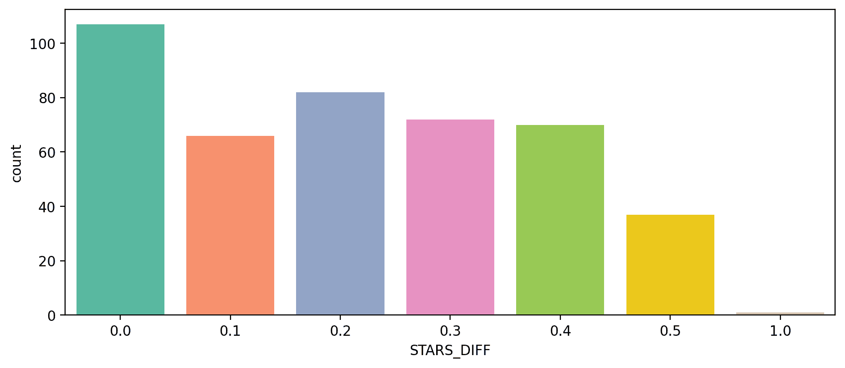 Some movies showed discrepancies of over 1.0 stars.
What movie had this close to 1 star differential?
fandango[fandango['STARS_DIFF'] >= 1]
🌐 4. Cross-Site Rating Comparison
4.1 Rotten Tomatoes: Critics vs Users
Scatterplot comparing critic ratings and user ratings:
plt.figure(figsize=(12,5))
sns.scatterplot(x='RottenTomatoes', y='RottenTomatoes_User', data=all_sites)
plt.show()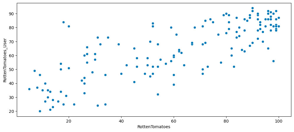 Plot the distribution of the differences between RT Critics Score and RT User Score:
all_sites['Rotten_Diff'] = all_sites['RottenTomatoes'] - all_sites['RottenTomatoes_User']
abs(Rotten_Diff).mean()
plt.figure(figsize=(12,4))
sns.histplot(data=Rotten_Diff,bins=30,kde=True)
plt.xlabel("Rotten_Diff")
plt.title("RT Critics Score minus RT User Score")
plt.show()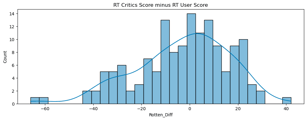
- Created a
Rotten_Diffvariable: Critics Score - User Score. - Measured and visualized the distribution.
Create a distribution showing the absolute value difference between Critics and Users on Rotten Tomatoes:
plt.figure(figsize=(12,4))

sns.histplot(data=abs(Rotten_Diff),bins=30,kde=True)

plt.xlabel("Rotten_Diff")

plt.title("Abs difference between RT Critics Score and RT User Score")

plt.show()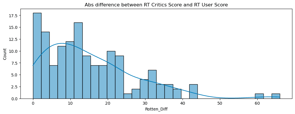
4.2 Metacritic Analysis
Scatterplot: Metacritic Critics vs Metacritic Users.
plt.figure(figsize=(12,5))

sns.scatterplot(x='Metacritic', y='Metacritic_User', data=all_sites)

plt.show()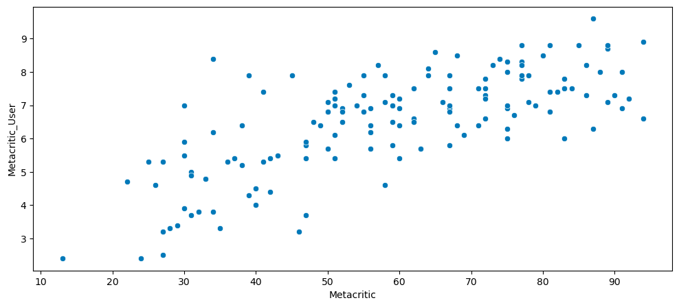
- Generally closer agreement than Rotten Tomatoes.
4.3 IMDb Analysis
Scatterplot of vote counts on Metacritic vs IMDb:
plt.figure(figsize=(12,5))

sns.scatterplot(x='Metacritic_user_vote_count', y='IMDB_user_vote_count', data=all_sites)

plt.show()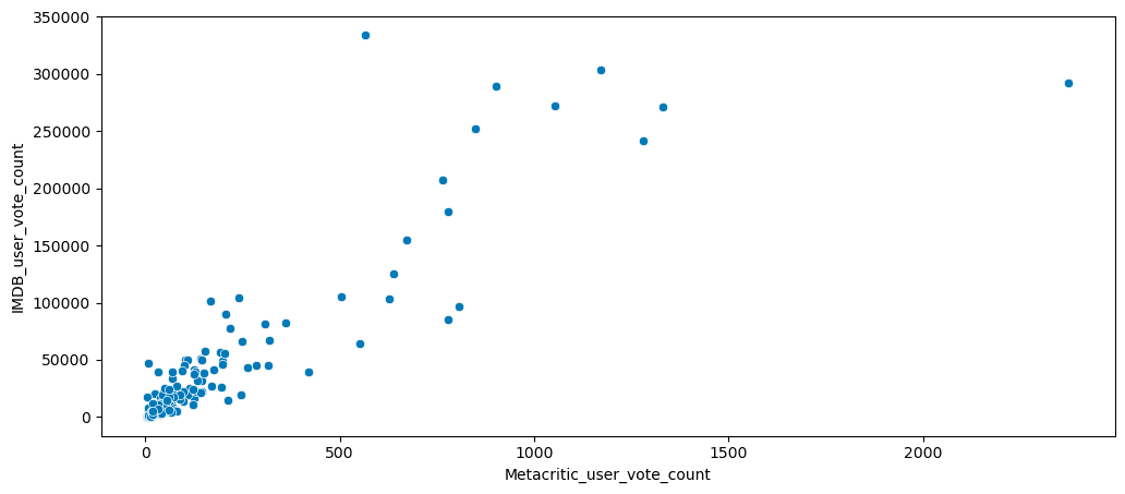
- Some outliers: movies with disproportionately high IMDb votes.
🔥 5. Normalizing Ratings Across Platforms
- To fairly compare Fandango against other platforms, all scores were normalized to a 0–5 scale
- Create a norm_scores DataFrame that only contains the normalizes ratings. Include both STARS and RATING from the original Fandango table
combined = pd.merge(fandango, all_sites, how='inner', on='FILM')
combined.head()
combined['RT_Norm'] = round(combined['RottenTomatoes'] / 20,1)

combined['RTU_Norm'] = round(combined['RottenTomatoes_User'] / 20,1)

combined['Meta_Norm'] = round(combined['Metacritic'] / 20,1)

combined['Meta_U_Norm'] = round(combined['Metacritic_User'] / 2,1)

combined['IMDB_Norm'] = round(combined['IMDB'] / 2,1)

combined.head()

norm_scores = combined[['STARS',"RATING",'RT_Norm','RTU_Norm','Meta_Norm','Meta_U_Norm','IMDB_Norm'|'STARS',"RATING",'RT_Norm','RTU_Norm','Meta_Norm','Meta_U_Norm','IMDB_Norm']]

norm_scores.head()
📈 6. Fandango vs Other Platforms
6.1 KDE Plot of Normalized Ratings
Comparing the overall distribution:
plt.figure(figsize=(15,6))

sns.kdeplot(data=combined, x='STARS',fill=True,clip=[0, 5],label='STARS')

sns.kdeplot(data=combined, x='RATING',fill=True,clip=[0, 5],label='Rating')

sns.kdeplot(data=combined, x='RT_Norm',fill=True,clip=[0, 5],label='RT_Norm')

sns.kdeplot(data=combined, x='RTU_Norm',fill=True,clip=[0, 5],label='RTU_Norm')

sns.kdeplot(data=combined, x='Meta_Norm',fill=True,clip=[0, 5],label='Meta_Norm')

sns.kdeplot(data=combined, x='Meta_U_Norm',fill=True,clip=[0, 5],label='Meta_U_Norm')

sns.kdeplot(data=combined, x='IMDB_Norm',fill=True,clip=[0, 5],label='IMDB_Norm')

plt.legend(loc='upper left')
Other way: Advantages: Advanced control!
Directly operate on ax (subplot object) instead of simply the current plot
Customize legend style, title, font size, border, etc.
Avoids legend misalignment when multiple subplots are used
def move_legend(ax, new_loc, **kws):
    old_legend = ax.legend_
    handles = old_legend.legendHandles
    labels = [t.get_text() for t in old_legend.get_texts()]
    title = old_legend.get_title().get_text()
    ax.legend(handles, labels, loc=new_loc, title=title, **kws)

fig, ax = plt.subplots(figsize=(15,6), dpi=150)
sns.kdeplot(data=norm_scores, clip=[0,5], fill=True, palette='Set1', ax=ax)
move_legend(ax, "upper left")
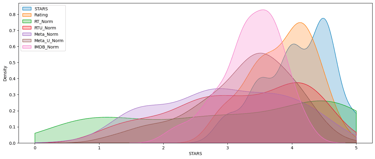 Clearly Fandango has an uneven distribution. We can also see that RT critics have the most uniform distribution. Let’s directly compare these two.
Create a KDE plot that compare the distribution of RT critic ratings against the STARS displayed by Fandango.
fig, ax = plt.subplots(figsize=(15,6),dpi=150)

sns.kdeplot(data=norm_scores[['RT_Norm','STARS'|'RT_Norm','STARS']],clip=[0,5],shade=True,palette='Set1',ax=ax)

move_legend(ax, "upper left")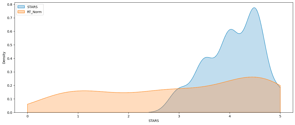
6.2 Histplot of Normalized Scores
Visualizing differences using histograms:
plt.figure(figsize=(15,6))

sns.histplot(data=norm_scores,bins=30)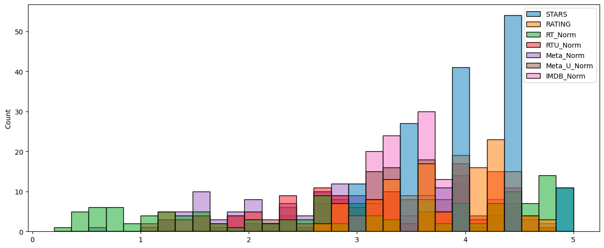
6.3 Clustermap of Normalized Scores
Clustering normalized ratings to reveal hidden patterns:
sns.clustermap(norm_scores,col_cluster=False)
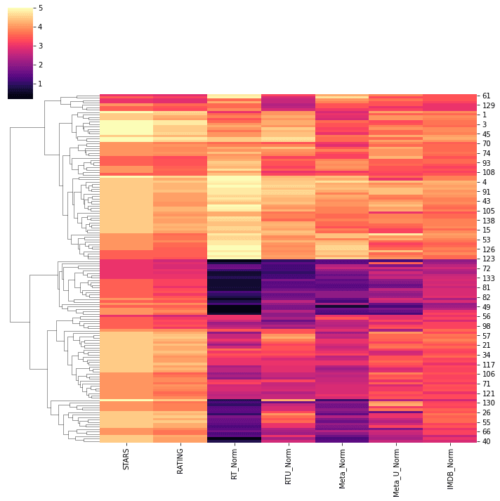 Poorly rated movies still appeared with higher Fandango stars.
🧪 7. Case Study: Top 10 Worst Movies
Identifying the 10 worst-rated movies by Rotten Tomatoes Critics and comparing across platforms:
norm_scores.nsmallest(10, 'RT_Norm')[['FILM', 'STARS', 'RT_Norm', 'Meta_Norm', 'IMDB_Norm'|'FILM', 'STARS', 'RT_Norm', 'Meta_Norm', 'IMDB_Norm']]KDE plot of their normalized ratings:
plt.figure(figsize=(15,6),dpi=150)

worst_films = norm_films.nsmallest(10,'RT_Norm').drop('FILM',axis=1)

sns.kdeplot(data=worst_films,clip=[0,5],shade=True,palette='Set1')

plt.title("Ratings for RT Critic's 10 Worst Reviewed Films")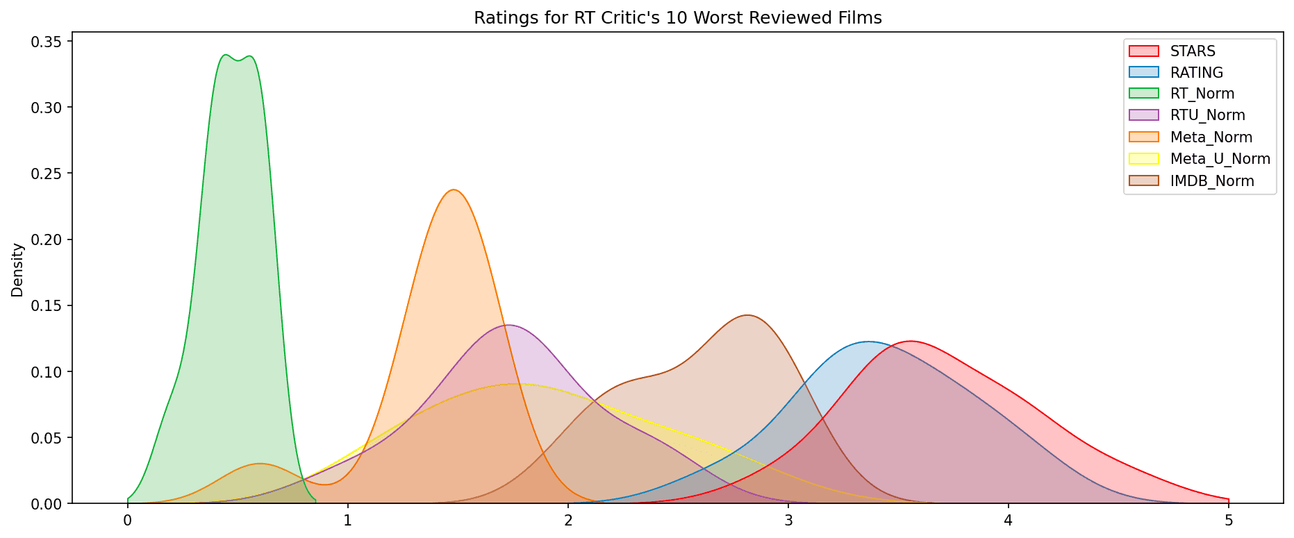
📌 Conclusion
-
Fandango’s displayed movie ratings were systematically biased upward in 2015.
-
The bias was consistent across genres and vote counts.
-
When compared to platforms like Rotten Tomatoes and Metacritic, Fandango ratings were notably inflated.
🚀 Future Directions
-
Analyze newer Fandango data (e.g., post-2019) to evaluate improvements.
-
Extend analysis to other online review sites such as Amazon, Yelp, or TripAdvisor.
-
Develop predictive models to estimate “true” ratings based on multi-platform consensus.
🙏 Acknowledgements
- Data Source: FiveThirtyEight’s Open Data Repository
- Inspiration: “Be Suspicious Of Online Movie Ratings”
- Tools: Python, Pandas, Seaborn, Matplotlib