2025-10-04 11:29 Tags:

Linear Regression — Gradients and Gradient Descent

1. Cost Function Reminder

We use Mean Squared Error (MSE):

$$J(\beta )=\frac{1}{2m}\sum _{j=1}^m{\left(y^j-{\hat{y}}^j\right)}^2$$

where:

• $m$ = number of samples
• $y^j$ = true value
• ${\hat{y}}^j={\sum }_{i=0}^n{\beta }_i{x}_i^j$ (prediction from our model)

---

2. Take Derivative (Gradient)

We want to minimize $J(\beta )$, so we take derivatives.

For one parameter ${\beta }_k$:

$$\frac{\partial J}{\partial {\beta }_k}=\frac{1}{m}\sum _{j=1}^m\left(y^j-\sum _{i=0}^n{\beta }_i{x}_i^j\right)(-x_k^j)$$

• This tells us how sensitive the cost is to changing ${\beta }_k$.
• If derivative is positive → cost increases as ${\beta }_k$ grows.
• If derivative is negative → cost decreases as ${\beta }_k$ grows.

---

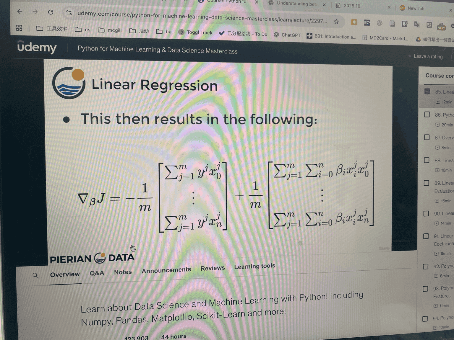
3. Gradient Vector

Instead of doing one parameter at a time, we collect all derivatives:

$${\nabla }_{\beta }J=\left[\begin{array}{c}\frac{\partial J}{\partial {\beta }_0}\\ \frac{\partial J}{\partial {\beta }_1}\\ ⋮\\ \frac{\partial J}{\partial {\beta }_n}\end{array}\right]$$

This is called the gradient.
It points in the direction of steepest increase of the cost.

---

$${\nabla }_{\beta }J=-\frac{1}{m}{X}^T(y-X\beta )$$

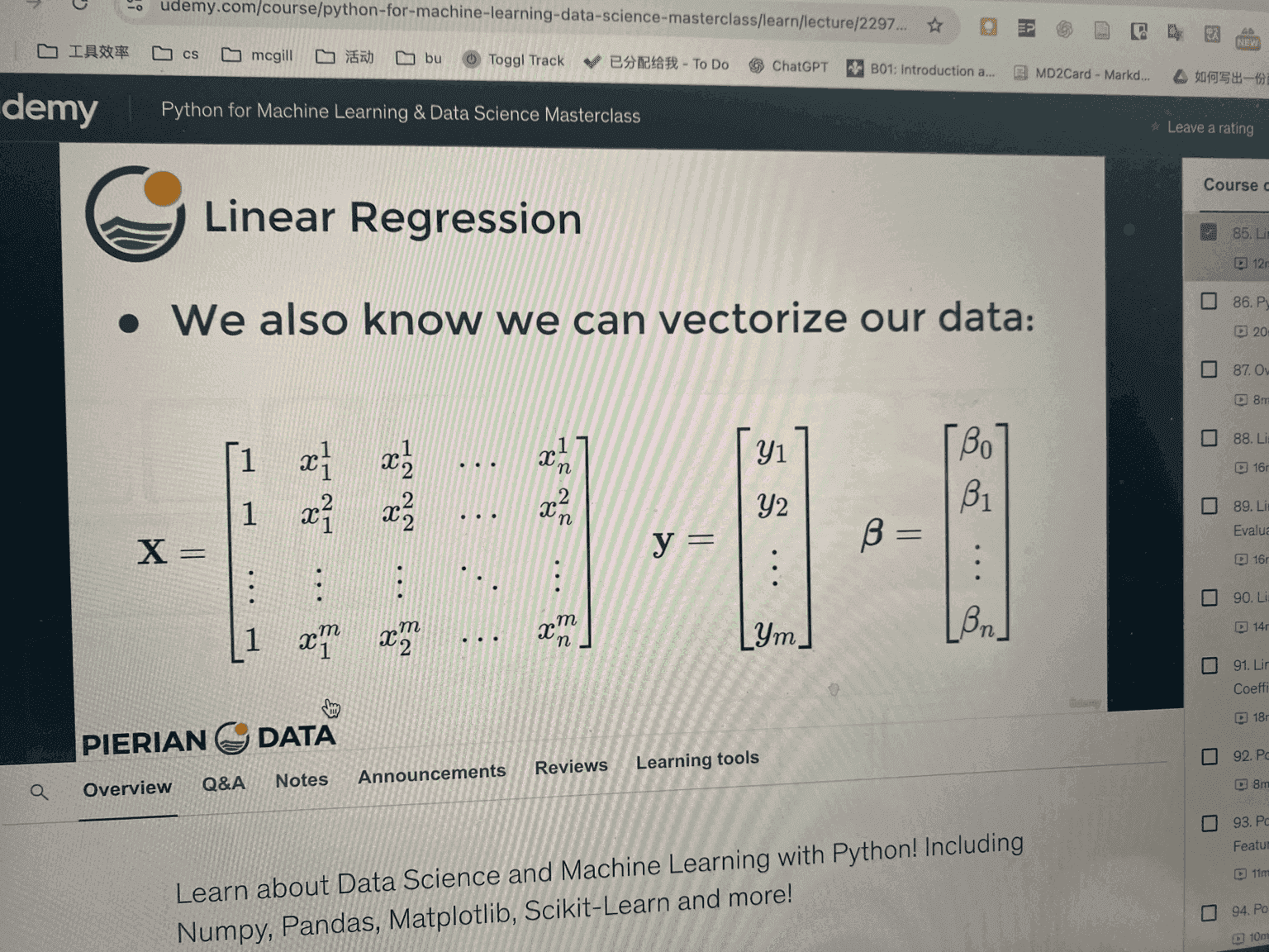
4. Matrix Form (Vectorization)

We can rewrite using matrices:

• $X$ = feature matrix (size $m\times (n+1)$, with 1’s column for intercept)
• $y$ = vector of actual outputs ($m\times 1$)
• $\beta$ = vector of parameters ($n+1\times 1$)

Prediction:

$$\hat{y}=X\beta$$

Gradient:

$${\nabla }_{\beta }J=-\frac{1}{m}{X}^T(y-X\beta )$$

This is a compact and efficient way to compute the gradient.

---

5. Gradient Descent Update Rule

We iteratively update:

$$\beta :=\beta -\eta {\nabla }_{\beta }J$$

• $\eta$ = learning rate (step size).
• We keep moving $\beta$ in the opposite direction of the gradient until convergence.

---

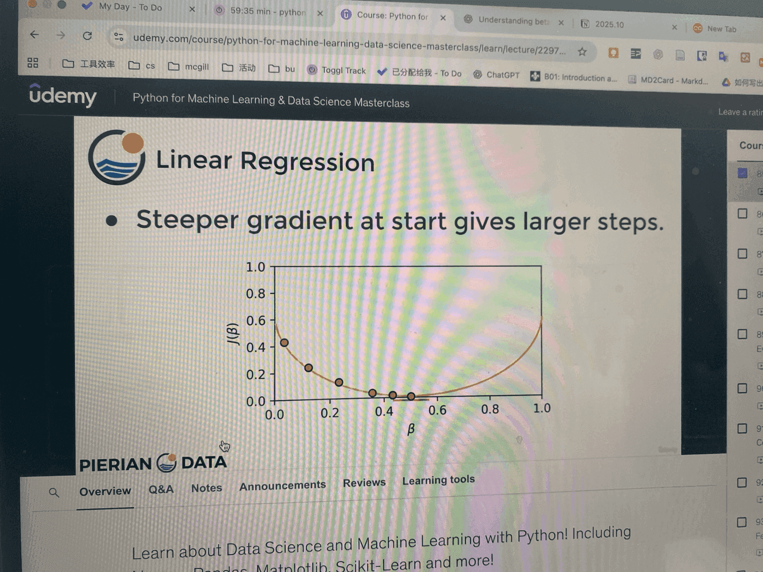
6. Intuition (Why Steps Change Size)

• At the start:
  Gradient is large → big steps downhill.

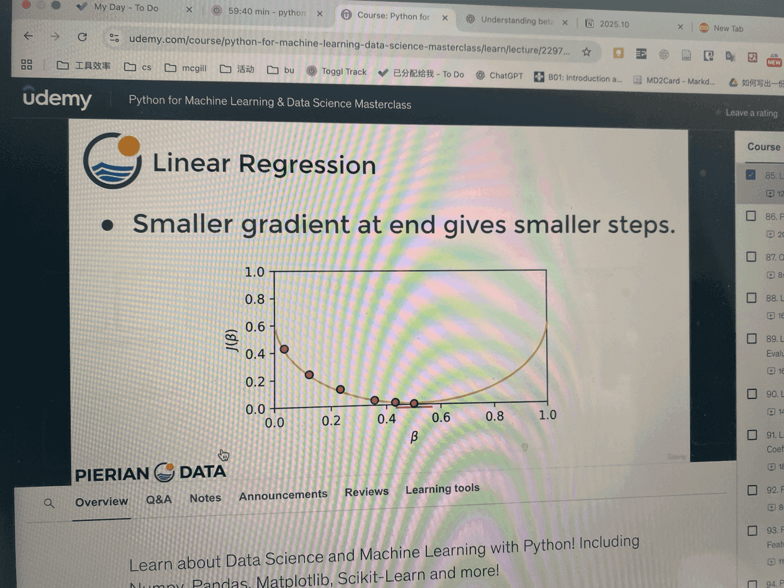
• Near the minimum:
  Gradient is small → smaller, finer steps.

So the algorithm naturally slows down as it gets closer to the best solution.

---

7. Algorithm Process

1. Initialize $\beta$ randomly (or zeros).
2. Compute gradient ${\nabla }_{\beta }J$.
3. Update $\beta :=\beta -\eta {\nabla }_{\beta }J$.
4. Repeat until convergence (cost stops decreasing).