2025-10-16 16:30 Tags:

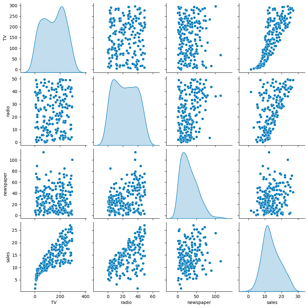
sns.pairplot(df, diag_kind='kde')

Helps visualize relationships and possible correlations between features.

Define Features & Target

X = df.drop('sales', axis=1)
# This is smart, just drop sales(y) you get all the features, instead of adding each one
y = df['sales']

Split Train/Test Data

from sklearn.model_selection import train_test_split
X_train, X_test, y_train, y_test = train_test_split(
    X, y, test_size=0.3, random_state=101)

Train the Model

from sklearn.linear_model import LinearRegression
model = LinearRegression()
model.fit(X_train, y_train)

• The model “learns” coefficients ( \beta_0, \beta_1, \beta_2, \beta_3 )

• Fit is based only on training data!

Evaluation on Test Set

Make Predictions

test_predictions = model.predict(X_test)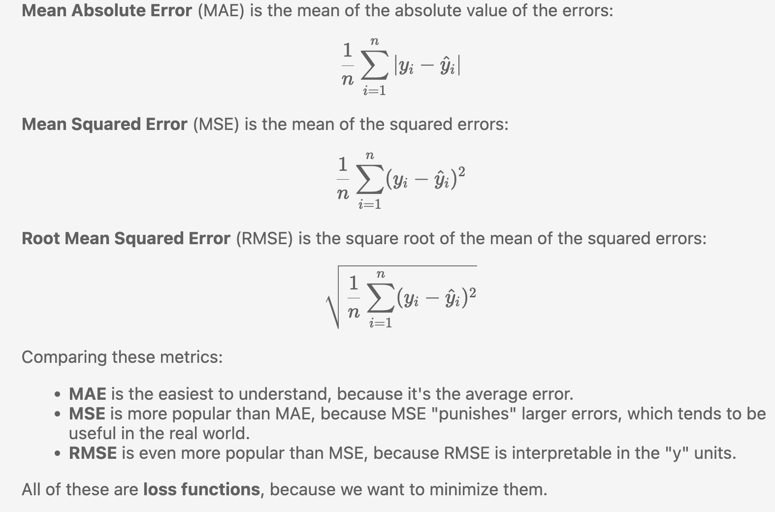

from sklearn.metrics import mean_absolute_error, mean_squared_error
MAE = mean_absolute_error(y_test, test_predictions)
MSE = mean_squared_error(y_test, test_predictions)
RMSE = np.sqrt(MSE)

✅ Lower MAE/MSE/RMSE → better fit
⚠️ Compare to df['sales'].mean() for perspective. MAE compare to mean(sales) MSE RMSE is too large, meaning the data may have outliers

---

Residual Analysis

Residual = Actual – Predicted You need to use residual plot to test whether it meets the linear relationship. It is the same as I was been taught in stats class! 4 assumptions of linearity

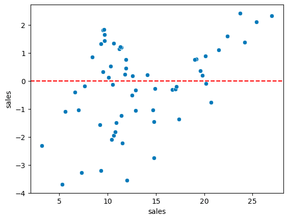
test_residual = y_test - test_predictions
 
sns.scatterplot(x=y_test,y=test_residual)
 
plt.axhline(y=0,color='r',ls='--')

Residuals should:

• Center around zero

• Have no clear pattern (homoscedasticity)

• Be approximately normal

sns.displot(test_residual,bins=25,kde=True)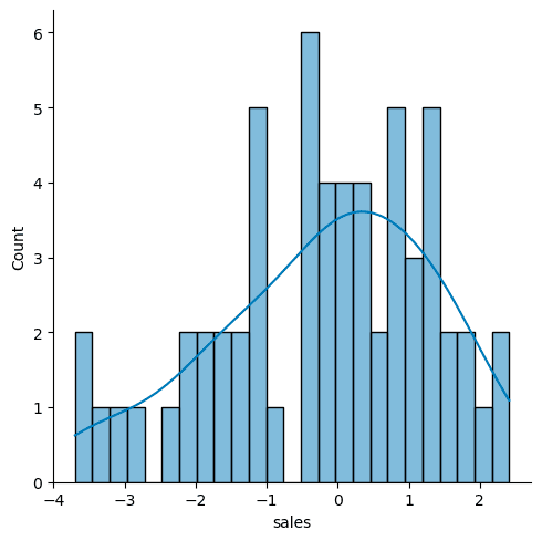

You can check with a Q-Q plot:

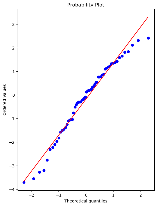
import scipy as sp
# Create a figure and axis to plot on
 
fig, ax = plt.subplots(figsize=(6,8),dpi=100)
 
# probplot returns the raw values if needed
 
# we just want to see the plot, so we assign these values to _
 
_ = sp.stats.probplot(test_residual,plot=ax)

---

Retrain on Full Data

After confirming model performance:

final_model = LinearRegression()
final_model.fit(X, y)

This uses all data for the final version of the model before deployment.

---

Coefficients

final_model.coef_

array([ 0.04576465, 0.18853002, -0.00103749])

• Holding all other features fixed, a 1 unit (A thousand dollars) increase in TV Spend is associated with an increase in sales of 0.045 “sales units”, in this case 1000s of units .

---

Making Predictions

campaign = [[149, 22, 12]]
final_model.predict(campaign)

dataset from outside to make new predictions

---

Saving & Loading Models

from joblib import dump, load
dump(final_model, 'sales_model.joblib')
loaded_model = load('sales_model.joblib')
loaded_model.predict(campaign)

Useful for deployment or reusing trained models later.

---

Summary Table

Step	Purpose	Key Function
Split data	Prevent overfitting	train_test_split
Train model	Learn parameters	LinearRegression().fit()
Predict	Generate output	.predict()
Evaluate	Measure accuracy	mean_absolute_error, mean_squared_error
Analyze residuals	Check assumptions	sns.displot, sp.stats.probplot
Save model	Reuse/deploy	joblib.dump()

---