11.2 Labels

The easiest place to start when turning an exploratory graphic into an expository graphic is with good labels. You add labels with the labs() function.

ggplot(mpg, aes(x = displ, y = hwy)) +
  geom_point(aes(color = class)) +
  geom_smooth(se = FALSE) +
  labs(
    x = 'Engine displacement (L)',
    y = 'Highway fuel economy (mpg)',
    color = 'car type',
    title = 'Fuel efficiency generally decreases with engine size',
    subtitle = 'Two seaters (sports cars) are an exception because of their light weight',
    caption = 'Data from fueleconomy.gov'
  )

se = FALSE: removes the shaded confidence interval around the line — we want a cleaner visual focus on the trend.

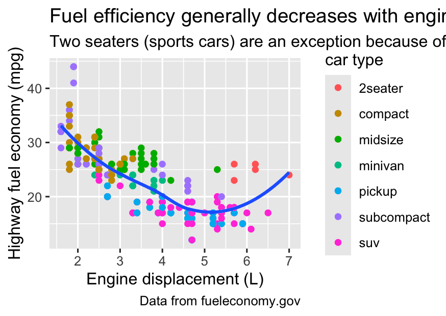
The purpose of a plot title is to summarize the main finding. Avoid titles that just describe what the plot is, e.g., “A scatterplot of engine displacement vs. fuel economy”. If you need to add more text, there are two other useful labels: subtitle adds additional detail in a smaller font beneath the title and caption adds text at the bottom right of the plot, often used to describe the source of the data.

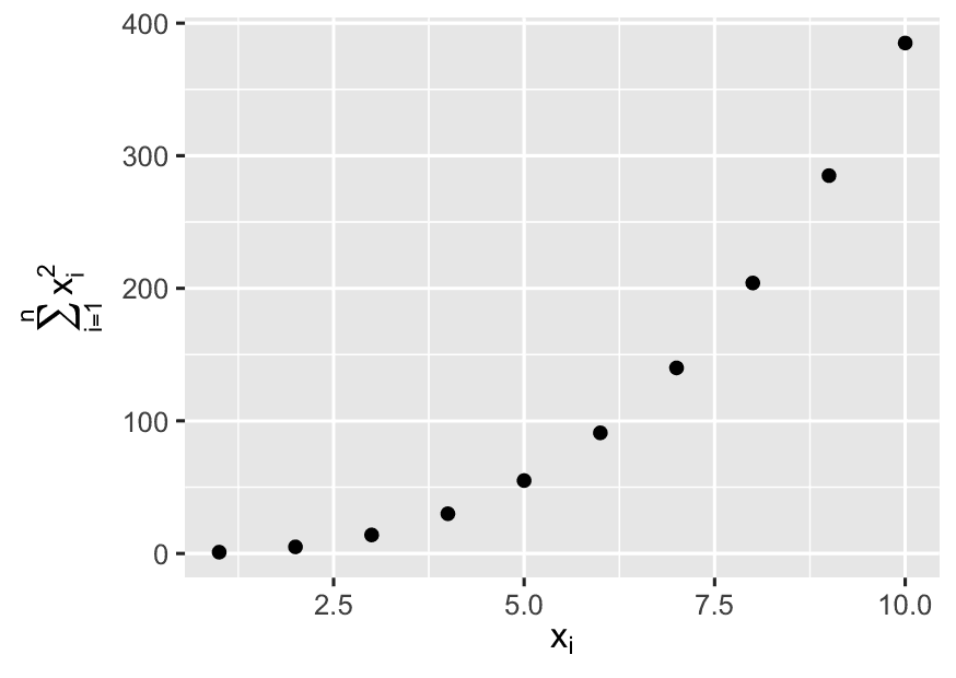
df <- tibble(
  x = 1:10,
  y = cumsum(x^2)
)
 
ggplot(df, aes(x, y)) +
  geom_point() +
  labs(
    x = quote(x[i]),
    y = quote(sum(x[i] ^ 2, i == 1, n))
  )

y = cumulative sum of squares: $y_1=1^2,y_2=1^2+2^2,\dots ,y_{10}={\sum }_{i=1}^{10}{x}_i^2$

What quote() does: It allows you to use plotmath expressions — that is, math-style annotations in R graphics. Here’s how they render:

• quote(x[i]) → displays as x₍ᵢ₎, meaning “x sub i”

• quote(sum(x[i] ^ 2, i == 1, n)) → displays as:

$$\sum _{i=1}^n{x}_i^2$$

This is a mathematical expression, like in textbooks, rendered on the plot using plotmath.

11.2.1 Exercises

1. Create one plot on the fuel economy data with customized title, subtitle, caption, x, y, and color labels.

ggplot(mpg, aes(x = displ, y = hwy, color = drv)) +
  geom_point(size = 2, alpha = 0.7) +
  geom_smooth(se = FALSE, method = "loess") +
  labs(
    title = "How Engine Size Affects Fuel Efficiency",
    subtitle = "Cars with larger engines tend to be less fuel efficient on highways",
    caption = "Data source: fueleconomy.gov | Visualization by YourName",
    x = "Engine Displacement (Liters)",
    y = "Highway Miles per Gallon (MPG)",
    color = "Drive Type"
  ) +
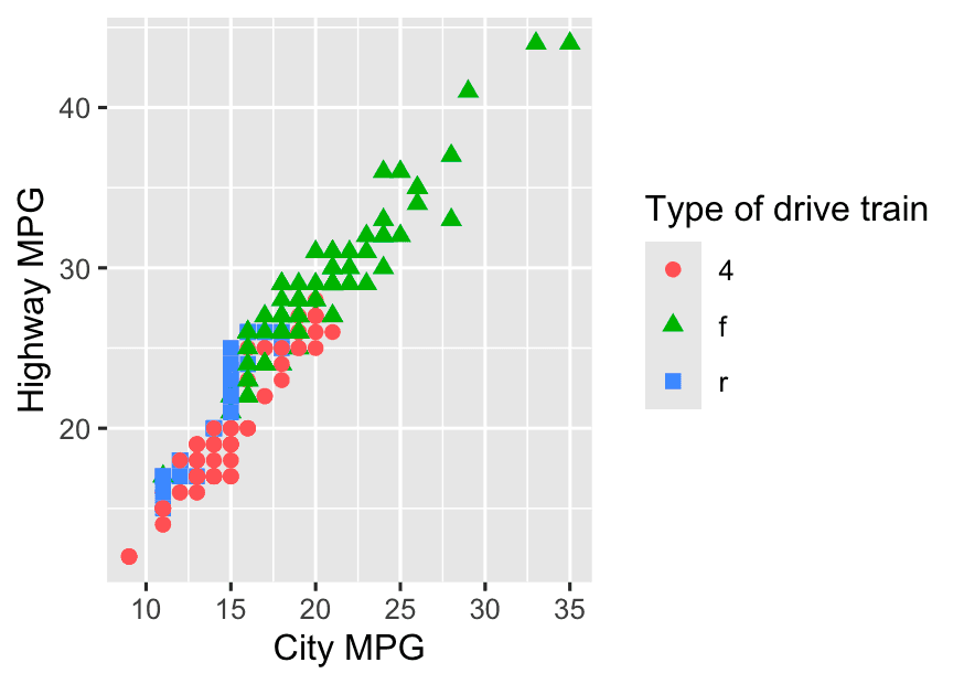
  theme_minimal()

2. Recreate the following plot using the fuel economy data. Note that both the colors and shapes of points vary by type of drive train.

ggplot(mpg, aes(x = cty, y = hwy, color = drv, shape = drv)) +
  geom_point(size = 2) +
  labs(
    x = "City MPG",
    y = "Highway MPG",
    color = "Type of drive train",
    shape = "Type of drive train"
  )

11.3 Annotations

In addition to labelling major components of your plot, it’s often useful to label individual observations or groups of observations. The first tool you have at your disposal is geom_text(). geom_text() is similar to geom_point(), but it has an additional aesthetic: label. This makes it possible to add textual labels to your plots.

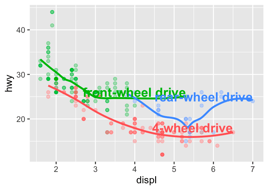
There are two possible sources of labels. First, you might have a tibble that provides labels. In the following plot we pull out the cars with the highest engine size in each drive type and save their information as a new data frame called label_info.

label_info <- mpg %>% 
  group_by(drv) %>% 
  arrange(desc(displ)) %>% 
  slice_head(n = 1) %>% #The car with the largest engine (`displ`)in each drive type (`drv`)
  mutate(
    drive_type = case_when(
      drv == 'f' ~ 'front-wheel drive',
      drv == 'r' ~ 'rear-wheel drive',
      drv == '4' ~ '4-wheel drive'
    )
  ) %>% 
  select(displ, hwy, drv, drive_type)

What is case_when()?

Think of case_when() as R’s version of a vectorized if-else ladder.

Here’s the logic:

case_when( condition1 ~ result1, condition2 ~ result2, ... )

It’s like saying:

“If drv is "f", then label it "front-wheel drive"; if it’s "r", then "rear-wheel drive", etc.”

The nice thing is: this works across a whole column (vectorized), not just one value.

ggplot(mpg, aes(x = displ, y = hwy, color = drv)) +
  geom_point(alpha = 0.3) +
  geom_smooth(se = FALSE) +
  geom_text(
    data = label_info,
    aes(x = displ, y = hwy, label = drive_type),
    fontface = "bold", size = 5, hjust = "right", vjust = "bottom"
  ) +
  theme(legend.position = "none")

• hjust = "right": aligns the label horizontally to the right of the point.

• vjust = "bottom": aligns vertically just below the point.

This is a precise way to annotate important points on the plot (like outliers or max engine cars per drive type).

theme(legend.position = "none")

• Removes the legend from the plot.

• Since you’re labeling the drive types directly on the plot, the legend becomes redundant.